


This section discusses the development of approaches to the ill-posed problem of blind deconvolution. First general deconvolution techniques assuming a known psf are presented. Then approaches for blind deconvolution with standard imaging systems are presented, along with a few means of accelerating their typically lengthy execution times.
Single Channel Multi-frame Blind Deconvolution
In 1972, Gerchberg and Saxton (GS) presented an algorithm “for the rapid solution of the phase of the complete wave function whose intensity in the diffraction and imaging planes of an imaging system are known.” The algorithm iterates back and forth between the two planes via Fourier transforms. The problem is constrained by the degree of temporal and/or spatial coherency of the wave.
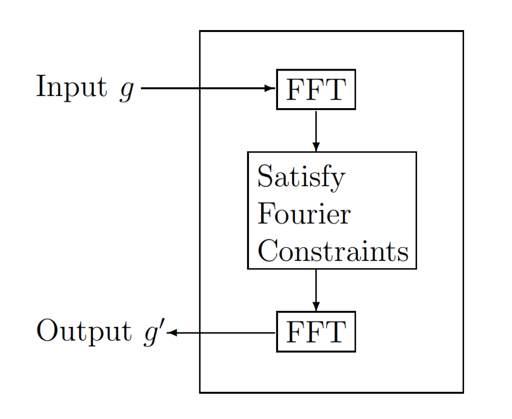
Additionally, the constraint of the magnitudes between the two planes results in a non-convex set in the image space according to Combettes. The algorithm is outlined in Figure 1.
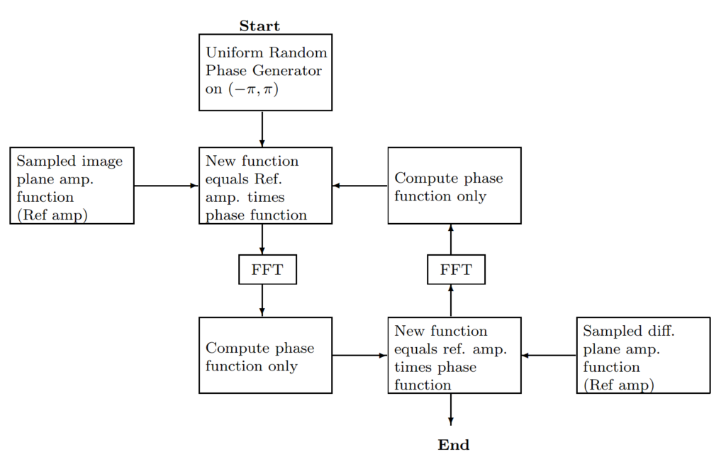
The inputs to the algorithm are the two input amplitude functions from the image and diffraction planes. A uniformly random phase generator is used to give the algorithm an initial starting point. GS offer a proof that the squared error between the results of the Fourier transforms and the input amplitude functions must decrease or remain the same on each iteration. They also point out that the solution reached is not unique.
In 1974, Lucy introduced another iterative technique based on increasing the likelihood of the observed sample each iteration. It is derived from Bayes’ Theorem and conserves the normalization and non-negativity constraints of astronomical images. The combination of both the Richardson algorithm and the Lucy algorithm is commonly referred to as the Richardson-Lucy (RL) algorithm.
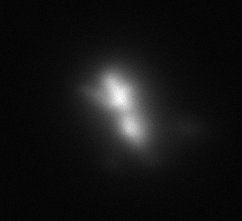
In 1982, Fienup compares iterative phase retrieval algorithms to steepest-descent gradient search techniques along with other algorithms. He discusses convergence rates and details some error functions for the algorithms. The first algorithm discussed is the error-reduction algorithm which is a generalized GS algorithm. It is applicable to the recovery of phase from two intensity measurements, like the GS algorithm, as well as one intensity measurement with a known constraint. In the area of astronomy, the known constraint is the non-negativity of the source object.
The error-reduction algorithm consists of the following four steps:
- Fourier transform gk(x) producing Gk(u)
- Make minimum changes in Gk(u) which allow it to satisfy the Fourier domain constraints producing G’k(u)
- Inverse Fourier transform G’k(u) producing g’k(x)
- Make minimum changes to g’k which allow it to satisfy the object domain constraints yielding gk+1(x)
where gk(x) and G’k(u) are estimates of f(x) and F(u), respectively.
For problems in astronomy with a single intensity image, the first three steps are identical to the first three steps of the GS algorithm. The fourth step applies the non-negativity constraint such that
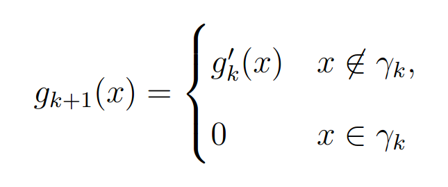
where γ is the set of points dependent on k, where g’k(x) violates the non-negativity constraint, i.e. where g’k(x) < 0.
For the case of a single intensity measurement with constraint, Fienup’s error measure is
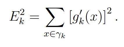
He found that the “error-reduction algorithm usually decreases the error rapidly for the first few iterations but much more slowly for later iterations.” He states that for the single image case convergence is “painfully slow” and unsatisfactory for that application.
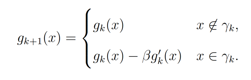
According to Fienup, a method proven to converge faster for both cases is the input-output (IO) algorithm. The IO algorithm differs from the error-reduction algorithm only in the object domain. The first three operations are the same for both algorithms. If those three operations are grouped together as shown in Figure 2 they can be viewed as a nonlinear system having input g and output g’. “The input g(x) no longer must be thought of as the current best estimate of the object; instead it can be thought of as the driving function for the next output, g'(x).”
The basic IO algorithm uses the following step to get the next estimate
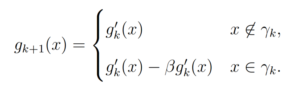
The output-output algorithm is a modified IO algorithm and uses the following step to get the next estimate
The hybrid IO algorithm uses the following step to get the next estimate
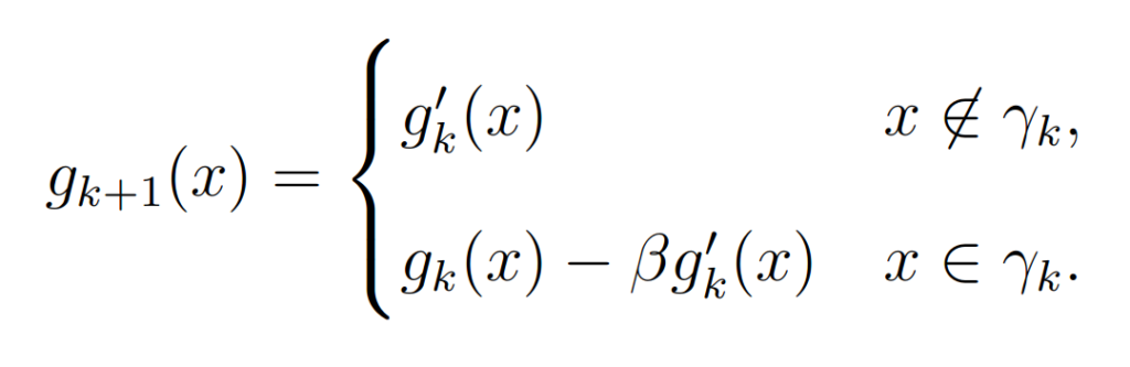
“The hybrid input-output algorithm is an attempt to avoid a stagnation problem that tends to occur with the output-output algorithm.” The output-output algorithm can stagnate with no means to get out of this state, but the hybrid input continues to grow until the output becomes non-negative.
Fienup analyzed the performance differences between the gradient search and the various IO algorithms for the case of phase retrieval from a single intensity image. Various values of β are used in the experiments. The optimal β value varied with the input and the algorithm. The hybrid seemed to have the best overall performance but was unstable and tends to move to a worse error before decreasing to a lower error than the other algorithms.